fftea

![]()
A simple and efficient FFT implementation.
Supports FFT of power-of-two sized arrays of real or complex numbers, using the Cooley-Tukey algorithm. Also includes some related utilities, such as windowing functions, STFT, and inverse FFT.
This package was built because package:fft is not actively maintained anymore, and wasn’t a particularly efficient implementation. There are a few improvements that make this implementation more efficient:
- The main FFT class is constructed with a given size, so that the twiddle factors only have to be calculated once. This is particularly handy for STFT.
- Doesn’t use a wrapper class for complex numbers, just uses a Float64x2List. Every little wrapper class is a seperate allocation and dereference. For inner loop code, like FFT’s complex number math, this makes a big difference. Float64x2 can also take advantage of SIMD optimisations.
- FFT algorithm is in-place, so no additional arrays are allocated.
- Loop based FFT, rather than recursive.
- Using trigonometric tricks to only calculate a quarter of the twiddle factors.
Usage
Running a basic real-valued FFT:
// myData.length must be a power of two. Eg 2, 4, 8, 16, ...
List<double> myData = ...;

final fft = FFT(myData.length);
final freq = fft.realFft(myData);
freq is a Float64x2List representing a list of complex numbers. See
ComplexArray for helpful extension methods on Float64x2List.
For efficiency, avoid recreating the FFT object each time. Instead, create one
FFT object of whatever size you need, and reuse it.
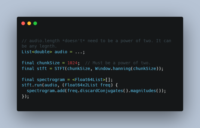
Running an STFT to calculate a spectrogram:
// audio.length *doesn't* need to be a power of two. It can be any legnth.
List<double> audio = ...;

final chunkSize = 1024;  // Must be a power of two.
final stft = STFT(chunkSize, Window.hanning(chunkSize));

final spectrogram = <Float64List>[];
stft.run(audio, (Float64x2List freq) {
  spectrogram.add(freq.discardConjugates().magnitudes());
});
The result of a real valued FFT is about half redundant data, so
discardConjugates removes that data from the result:
[sum term, …terms…, nyquist term, …conjugate terms…] ^—– These terms are kept ——^ ^- Discarded -^
Then magnitudes discards the phase data of the complex numbers and just keeps
the amplitudes, which is usually what you want for a spectrogram.
If you want to know the frequency of one of the elements of the spectrogram, use
stft.frequency(index, samplingFrequency), where samplingFrequency is the
frequency that audio was recorded at, eg 44100. The maximum frequency (aka
nyquist frequency) of the spectrogram will be
stft.frequency(chunkSize / 2, samplingFrequency).
See the example for more detailed usage.
Benchmarks
I found some other promising FFT implementations, so I decided to benchmark them too: scidart, and smart_signal_processing.
To run the benchmarks:
- Go to the bench directory and pub get,
cd bench && dart pub get - Run
dart run bench.dart
fftea gains some of its speed by caching the twiddle factors between runs, and by doing the FFT in-place. So the benchmarks are broken out into cached and in-place variants. Caching and running in-place is also applied to some of the other libraries, where appropriate.
In the table below, “cached” means the construction of the FFT object is not included in the benchmark time. And “in-place” means using the in-place FFT, and the conversion and copying of the input data into whatever format the FFT wants is not included in the benchmark. Run in Ubuntu on a Dell XPS 13.
| Size | package:fft | smart | smart, in-place | scidart | scidart, in-place* | fftea | fftea, cached | fftea, in-place, cached |
|---|---|---|---|---|---|---|---|---|
| 16 | 410.6 us | 28.3 us | 8.3 us | 347.2 us | 164.0 us | 42.2 us | 11.6 us | 10.9 us |
| 64 | 416.4 us | 8.2 us | 2.7 us | 169.0 us | 194.0 us | 73.5 us | 41.6 us | 41.8 us |
| 256 | 470.6 us | 14.0 us | 11.0 us | 904.9 us | 812.8 us | 34.1 us | 8.4 us | 6.1 us |
| 2^10 | 1.54 ms | 47.2 us | 44.1 us | 8.28 ms | 8.26 ms | 36.3 us | 30.5 us | 27.3 us |
| 2^12 | 7.65 ms | 206.1 us | 197.3 us | 132.99 ms | 121.27 ms | 159.2 us | 143.9 us | 129.3 us |
| 2^14 | 39.83 ms | 940.1 us | 899.4 us | 1.96 s | 1.96 s | 750.1 us | 695.5 us | 590.2 us |
| 2^16 | 261.38 ms | 6.04 ms | 5.62 ms | 41.44 s | 41.60 s | 4.71 ms | 5.89 ms | 3.56 ms |
| 2^18 | 1.31 s | 27.65 ms | 27.84 ms | Skipped | Skipped | 20.80 ms | 24.92 ms | 15.66 ms |
| 2^20 | 7.29 s | 168.84 ms | 151.12 ms | Skipped | Skipped | 119.93 ms | 106.00 ms | 88.26 ms |
In practice, you usually know how big your FFT is ahead of time, so it’s pretty easy to construct your FFT object once, to take advantage of the caching. It’s sometimes possible to take advantage of the in-place speed up too, for example if you have to copy your data from another source anyway you may as well construct the flat complex array yourself. Since this isn’t always possible, the “fftea, cached” times are probably the most representative. In that case, fftea is about 60-80x faster than package:fft, and about 30% faster than smart_signal_processing. Not sure what’s going on with scidart, but it seems to be O(n^2).
* Scidart’s FFT doesn’t have an in-place mode, but they do use a custom format, so in-place means that the time to convert to that format is not included in the benchmark.